1.Statistical Analyses of Parameters for Low-Resolution Part

(1). Distributions of Atmospherical Parameters (Teff, logg, [Fe/H]) and Radial Velocity (rv)

The atmospherical parameter distribution of DR6_v2 is shown as follows. Metallicity bins are represented by different colors.

The following diagrams show the distributions of errors of atmospherical parameters (Teff, logg, [Fe/H]) as well as rv in different SNR of r band (snr)) bins. These parameters are estimated by LASP.

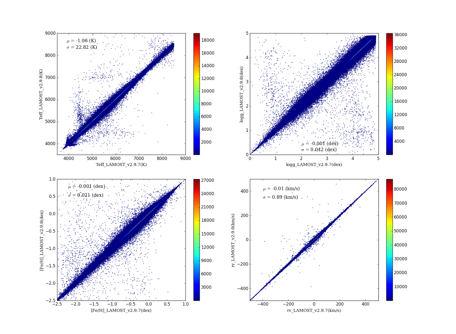
(2). The Comparison between DR6_v2 (the international version) and DR6_v1 (the domestic version)

LAMOST DR6_v1 was released in March of 2019, which is available to domestic users. Comparing DR6_v1, some improvements have been made for the DR6_v2. We compare the atmospherical parameters and rv of DR6_v2 with those of DR6_v1. There are some differences between these two versions, which can seen in the following figures. The x-axis represents parameters from DR6_v1, and y-axis for DR6_v2.

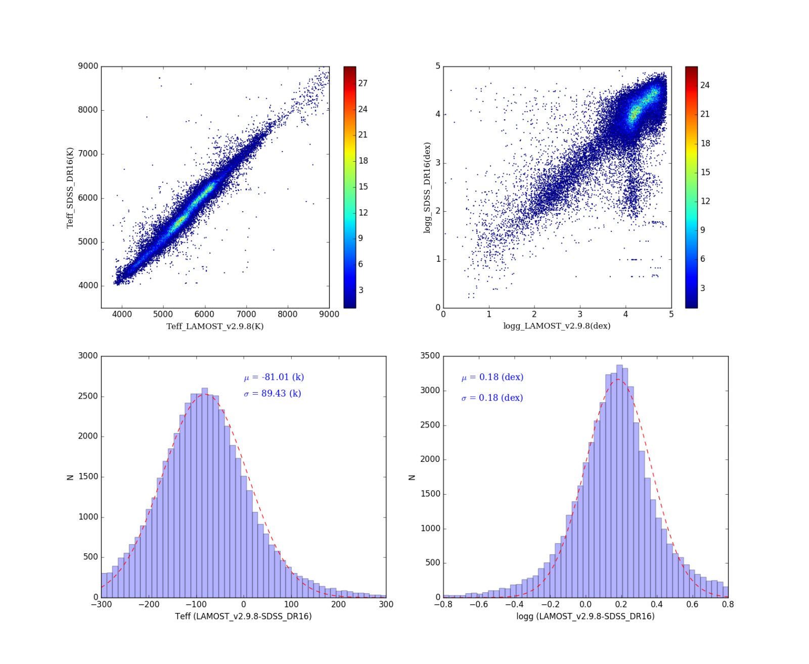
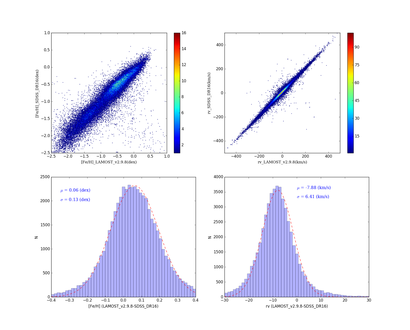
(3). The Parameter Comparisons between DR6_v2 Low-resolution Part and SDSS DR16

The following figures show the comparisons of atmospherical parameters (Teff, logg, [Fe/H]) as well as rv between DR6_v2 low-resolution data and SDSS DR16. The mean values and the standard deviations of the differences are also plotted in the figures. For the parameters of logg, a branch is seen in the top-right panel. It could be explained by the inhomogeneous distribution of the atmospherical parameters in the ELODIE library. There is a hole for giants in the ELODIE library, making the estimations of the initial guess for atmospherical parameters in the giant hole inaccurate.

2. Statistical Analyses of Parameters for Medium-Resolution Part

(1).Distributions of Error of Atmospherical Parameters (Teff, logg, [Fe/H]) and Radial Velocity (rv) for the combined spectra

The following figures show the distributions of error of atmospherical parameters (Teff, logg, [Fe/H]) and rv for the combined spectra. There are four kinds of values of rv that are estimated by different methods. The errors of parameters are divided into four groups according to the snr, presented by different colors.

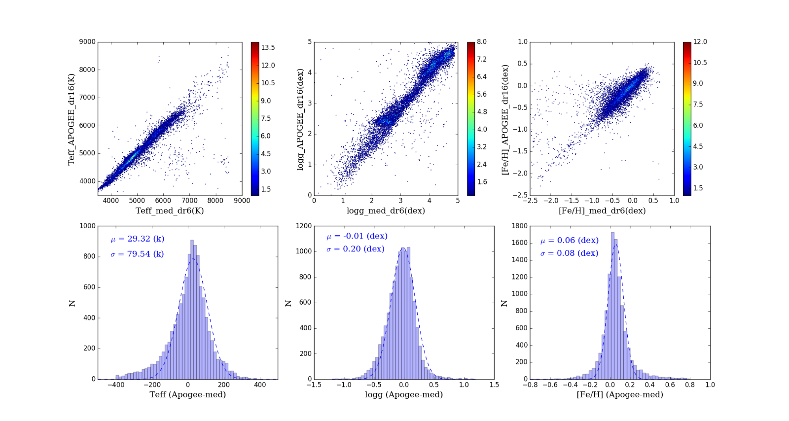
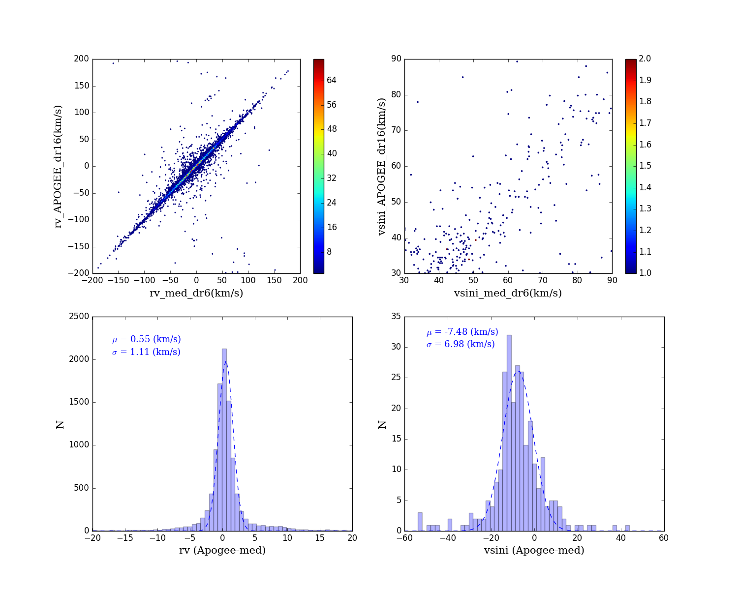
(2).The Parameter Comparisons between DR6_v2 Medium-resolution Part and APOGEE

The comparisons of atmospherical parameters (Teff, logg, [Fe/H]), rv and vsini between DR6_v2 Medium-resolution data and AOPGEE are shown in the following figures. We also plot the mean values and the standard deviations of the differences of the parameters in the figures.

(3).Distribution of [α/M]

[α/M] is estimated by the convolutional neural network (CNN) method. The [M/H]-[α/M] diagram and the histogram of [α/M] derived from combined spectra are shown in the following figure